Identify Differences In Columns In Excel For Mac

Microsoft Excel Office software has a range of features that enable the user to create worksheets according to their needs and requirements. It is easy to create a macro to compare columns to find missing data in Excel. Macros in Excel can be used to do calculations and data manipulations in the worksheets. It is not required to write Excel macros from scratch as there are many resources available on the web that provide code for macros. Knowledge of programming may prove helpful but is not essential to create a macro to compare columns to find missing data in Excel Worksheets. Solution If the macro finds the missing data, what do you want to do with it?

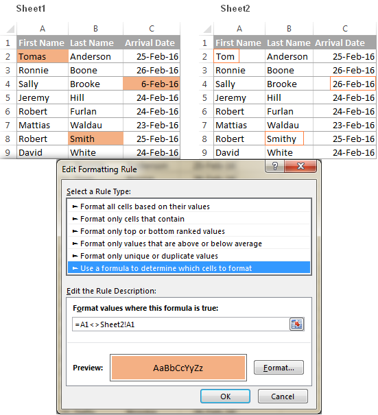
In my macro, the data in column D of sheet C which is missing in the same column of sheet Q will be marked yellow. This may or may not be what you want to do with the missing data. Here is the macro below. Dolphin emulator controller setup. Modify it with whatever you want. First run the macro and look at sheet C to see what happens before modifying the macro: Sub test() Dim cfindq As Range, rc As Range, cc As Range, x As Double On Error Resume Next With Worksheets('c').Cells.Interior.ColorIndex = xlNone Set rc = Range(.Range('d2'),.Range('d2').End(xlDown)) For Each cc In rc x = cc.Value With Worksheets('q').Columns('D:D') Set cfindq =.Cells.Find(what:=x, lookat:=xlWhole) If cfindq Is Nothing Then GoTo line1 Else GoTo line2 End If End With line1: cc.Interior.ColorIndex = 6 line2: Next cc End With End Sub Note Thanks to for this tip on the forum.

This step-by-step article describes how to find data in a table (or range of cells) by using various built-in functions in Microsoft Excel. You can use different formulas to get the same result. Excel for Mac 2011 is always trying to tell you what it can do. When you’re in a worksheet, the cursor changes as you move the mouse around. The cursor’s appearance reveals what you can do: Open cross: This is the mouse cursor you see most of the time in Excel. When you see the open cross, Excel expects you to do something.

The easiest way to combine list of values from a column into a single cell I have found to be using a simple concatenate formula. 1) Insert new column 2) Insert concatenate formula using the column you want to combine as the first value, a separator (space, comma, etc) as the second value, and the cell below the cell you placed the formula in as the third value.

3) Drag the formula down through the end of the data in the column of interest 4) Copy & paste special values in the newly created column to remove the formulas, and BOOM!all values are now in the top cell. For example, the following formula will combine all values listed in column A in cell C3 with a semi-colon separating them =CONCATENATE(A3,';',C4).